Discop: 基于分布副本的可证明安全隐写 (S&P 2023)

论文标题:Discop: Provably Secure Steganography in Practice Based on “Distribution Copies”
中文版
隐写安全性
在隐写领域,可证明安全的追求由来已久。
1949 年,信息学科祖师爷 Claud Shannon 在其经典论文 Communication Theory of Secrecy Systems 中开宗明义地指出了构建隐蔽系统的困难性。直到二十世纪九十年代,学界开始模仿密码学中的安全性定义来定义隐写的安全性。1998 年,Christian Cachin 给出了隐写的信息论安全 (information-theoretic security) 定义,使用载体数据分布 $P_{\mathrm{c}}$ 和载密数据分布 $P_{\mathrm{s}}$ 之间的 KL 散度 $D_{\mathrm{KL}}\left(P_{\mathrm{c}}\|P_{\mathrm{s}} \right)$ 来建模隐写安全性——KL 散度越小,$P_{\mathrm{c}}$ 和 $P_{\mathrm{s}}$ 越接近,敌手做出错误判断的概率就越大,隐写系统也越安全。如果 $D_{\mathrm{KL}}\left(P_{\mathrm{c}}\|P_{\mathrm{s}} \right)\le\epsilon$,则称隐写系统是 $\epsilon$-安全的;如果 $\epsilon=0$ ,则称隐写系统是绝对安全的 (perfectly secure) ,在这种情况下,$P_{\mathrm{c}}$ 和 $P_{\mathrm{s}}$ 严格相等,敌手判断一个对象是载体还是载密的能力无法好于随机猜测。2002 年,图灵奖得主 Manuel Blum 团队的 Nicholas Hopper 、John Langford 和 Luis von Ahn 在美密会上给出了隐写的计算安全 (computational security) 定义,他们假设敌手在玩一个判断某个对象是载体还是载密的区分游戏,如果所有概率多项式时间 (PPT) 敌手的攻击优势都关于安全参数可忽略 (negligible) ,则认为隐写系统是安全的。
Definitions:
- 载体 (cover) : an object without a secret message embedded
- 载密 (stego) : an object with a secret message embedded
References:
- C. E. Shannon. Communication Theory of Secrecy Systems. BSTJ ’49
- C. Cachin. An Information-Theoretic Model for Steganography. IH ’98
- N. J. Hopper et al. Provably Secure Steganography. CRYPTO ’02
闲聊:Christian Cachin 是 IACR Fellow ,是 Cryptology ePrint Archive (可理解为密码学界的 arXiv) 的发起人之一。Luis von Ahn 是验证码 CAPTCHA 的发明人之一 (第一作者) 、多邻国 Duolingo 的创始人之一。
为什么需要可证明安全隐写

可参考《可证安全隐写:理论、应用与展望》第 1 节:隐写的经验安全与可证安全。
……
对于一个经验安全的隐写算法来说,攻击者总是会存在一个可观的优势,哪怕它比较小。因而对隐写者来说,用这个隐写工具的时候,确实有很大风险,因为攻击者通过一定的数据量就能以非常高的信心来识别他。隐写者就会思考,如何使得攻击者的优势为零,或者使攻击者的优势可以忽略。这其实就对应可证安全隐写。如果我们不对攻击者的计算能力加限定,对于任意计算能力的攻击者,都能保证其获得的优势为零,这就是信息论安全。如果退一步,对限定计算能力的攻击者能保证他能获得的优势可忽略,这就是计算安全隐写。
现有可证明安全隐写构造及其在实践中的问题
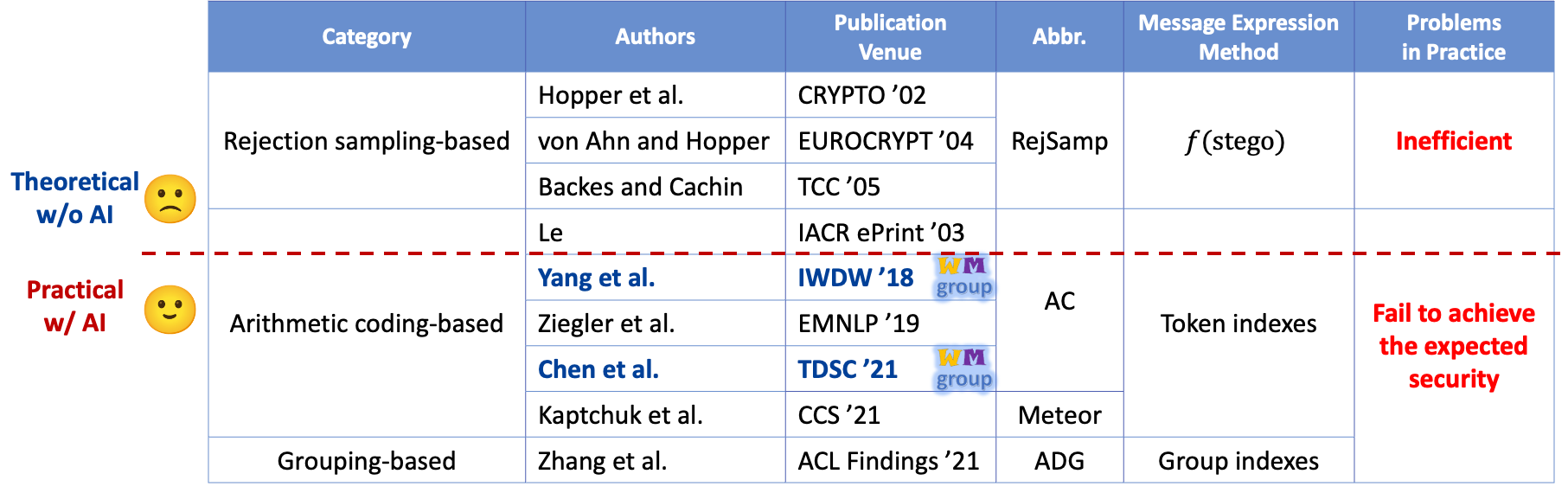
自隐写安全性的定义提出以来,研究者们相继提出了几种追求可证明安全的隐写构造。我们分析了它们在实践中的问题。
- 基于拒绝采样的构造:时间消耗的期望随着嵌入消息长度呈指数增长;当分布的最小熵非常小时,拒绝采样算法极易失败。
- 基于算术编码的构造:任意消息的概率都有 $2^{-l}\left(l\in \mathbb{N} \right)$ 的形式,相应地,载密也有 $2^{-l}$ 的形式。然而,模型预测出的载体数据分布几乎不可能与这种载密数据分布恰好匹配,这使得消息嵌入算法需要对载体数据分布进行调制,从而引入失真。为了减少失真,可以简单地通过填充来增加消息长度,使得载体数据的概率变得更小,更接近某个 $2^{-l}$ ;随着消息长度接近无穷大,失真趋于 0 ,这显然是不切实际的;即便如此,引入的失真是关于消息长度 (而非安全参数) 的可忽略函数,使得这种构造无法达到预期的安全性。
- 基于分组的构造:当且仅当分组是完美平衡时,这种构造是安全的。然而,离散概率分布难以平衡分组,使得这种构造无法达到预期的安全性。
References:
- N. J. Hopper et al. Provably Secure Steganography. CRYPTO ’02
- L. von Ahn and N. J. Hopper. Public-Key Steganography. EUROCRYPT ’04
- M. Backes and C. Cachin. Public-Key Steganography with Active Attacks. TCC ’05
- T. V. Le. Efficient Provably Secure Public Key Steganography. Cryptology ePrint Archive ’03
- K. Yang et al. Provably Secure Generative Steganography Based on Autoregressive Model. IWDW ’18
- Z. Ziegler et al. Neural Linguistic Steganography. EMNLP ’19
- K. Chen et al. Distribution-Preserving Steganography Based on Text-to-Speech Generative Models. TDSC ’21
- G. Kaptchuk et al. Meteor: Cryptographically Secure Steganography for Realistic Distributions. CCS ’21
- S. Zhang et al. Provably Secure Generative Linguistic Steganography. ACL Findings ’21
基于分布副本的可证明安全隐写构造
在本文中,我们提出新的基于分布副本的可证明安全隐写构造。
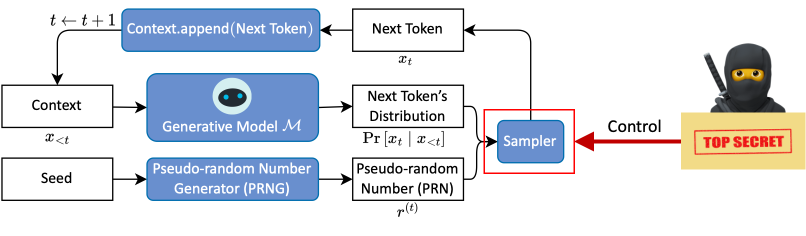
我们以文本生成任务为例来介绍提出的隐写构造,这类任务一般使用自回归模型 (auto-regressive model) 如 GPT 系列模型,一个 token 一个 token 地生成文本。具体地,给定一个上文 (context) 作为输入,自回归模型会预测下一个 token 的概率分布 $\mathcal{P}^{(t)}=\Pr \left[x_{t}\mid x_{<t} \right]$ ,然后从这个概率分布中随机采样 (random sampling) 出一个 token,作为下一个 token 追加到上文的尾部。重复预测和随机采样,直至达到终止条件。
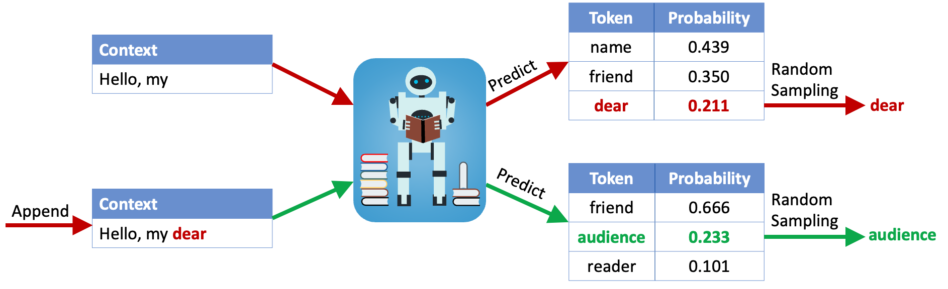
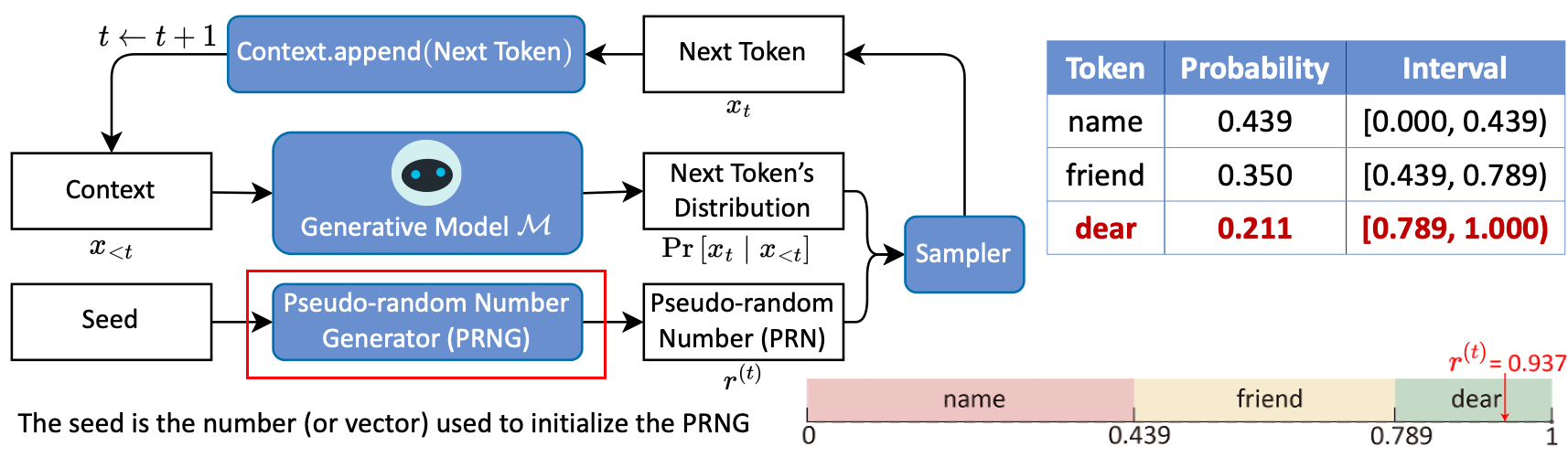
随机采样一般通过以下步骤实现:
- 在 $\left[0,1 \right)$ 上,根据 $\mathcal{P}^{\left(t \right)}$ 为所有候选 token 分配互不相交的左闭右开区间,每个 token 对应的区间长度等于这个 token 被选中的概率;
- 消耗一个由伪随机数生成器 (PRNG) 生成的伪随机数 (PRN) $r^{\left(t \right)}$ ,选取 $r^{\left(t \right)}$ 落入的区间对应的 token 作为下一个 token 。
举例:假设 $r^{\left(t \right)}=0.937$ ,因为其落入 dear 对应的区间,所以选取 dear 作为下一个 token 。
在生成过程中,如何安全地嵌入消息?
我们认为这个问题的答案是,在秘密消息的控制下进行采样,这种采样需要满足两个条件:
- 不可区分 (indistinguishable) :隐写采样应与随机采样不可区分;
- 可逆 (reversible) :接收方可以将收到的 token 译码为秘密消息。
基础构造
我们观察到,对于一个候选 token 数量大于 1 的概率分布来说,区间分配方案并不是唯一的。
这样,给定一个概率分布,我们可以为其创建多个分布副本 (distribution copies) ,然后使用分布副本的索引值 (index) 来表达消息。
我们通过循环移位 (rotate) 来创建分布副本。为了方便理解,这里给出一个实例。
假设概率分布为:
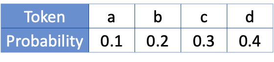
不妨以 a-b-c-d 顺序排列的分配方案作为作为初始区间分配方案,即分布副本 0。
若要嵌入 1 比特消息,则需要创建 $2^{1}=2$ 个分布副本,对应的移位步长为 $1/2=0.5$ 。
将分布副本 0 循环移位 0.5 ,可得到分布副本 1。
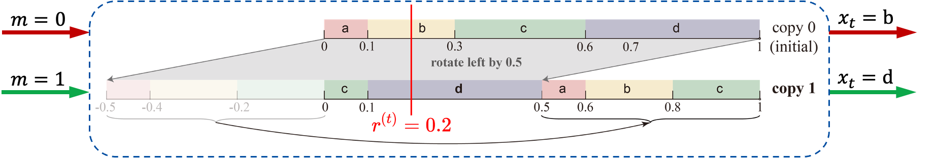
假设 PRNG 生成的 PRN $r^{\left(t \right)}=0.2$ 。
- 若消息 $m=0$ ,则从分布副本 0 采样,因为 $r^{\left(t \right)}$ 落入 b 对应的区间,所以采出 b 作为下一个 token ;
- 若消息 $m=1$ ,则从分布副本 1 采样,因为 $r^{\left(t \right)}$ 落入 d 对应的区间,所以采出 d 作为下一个 token 。
🤔️接收方如何提取消息?
如果接收方与发送方共享相同的上文、生成模型,他就可以拿到相同的概率分布;相似地,如果接收方与发送方共享相同的种子、PRNG,他就可以拿到相同的 PRN 。
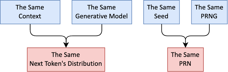
这样,接收方可以与发送方同步相同的状态,并通过判断收到的 token 是从哪个分布副本采样得到的来提取消息。

唯一译码条件、争议区间与嵌入率
如何保证接收方能正确提取消息?能嵌入多长消息?
不难推出,当且仅当消耗的 PRN 在所有分布副本中落入的区间对应的 token (下文简称「落入的 token」) 互不相同时,这次采样可以唯一地表达消息。
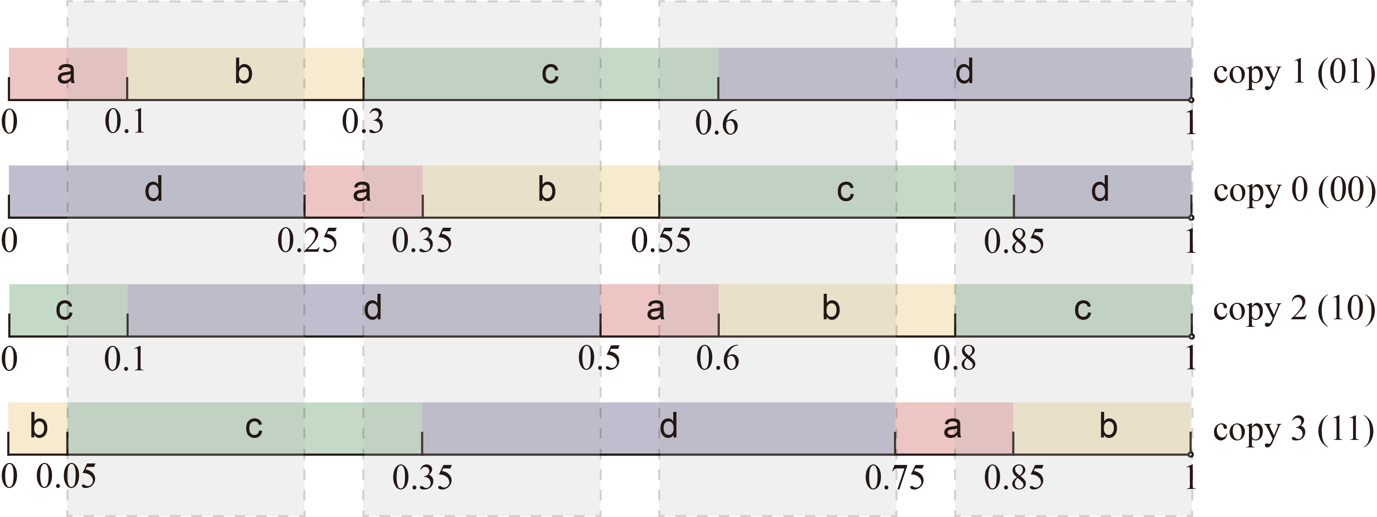
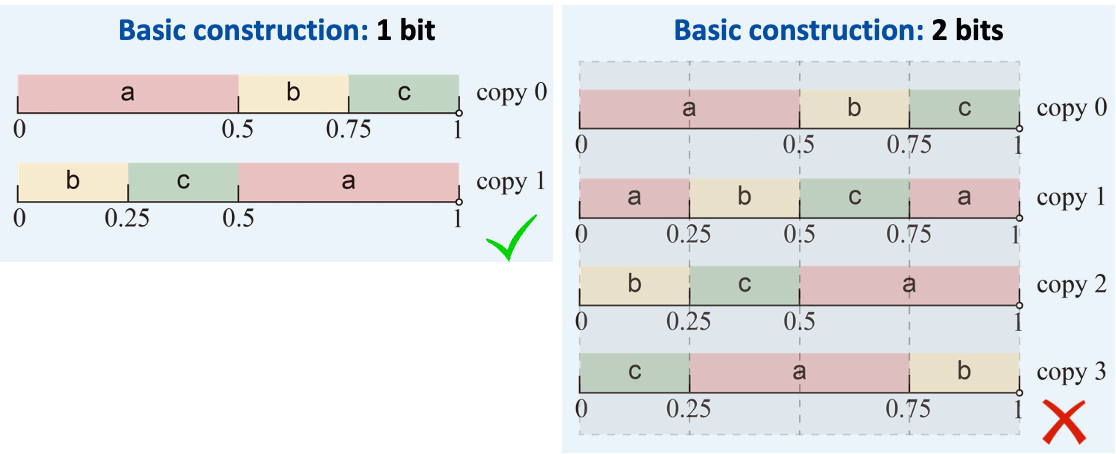
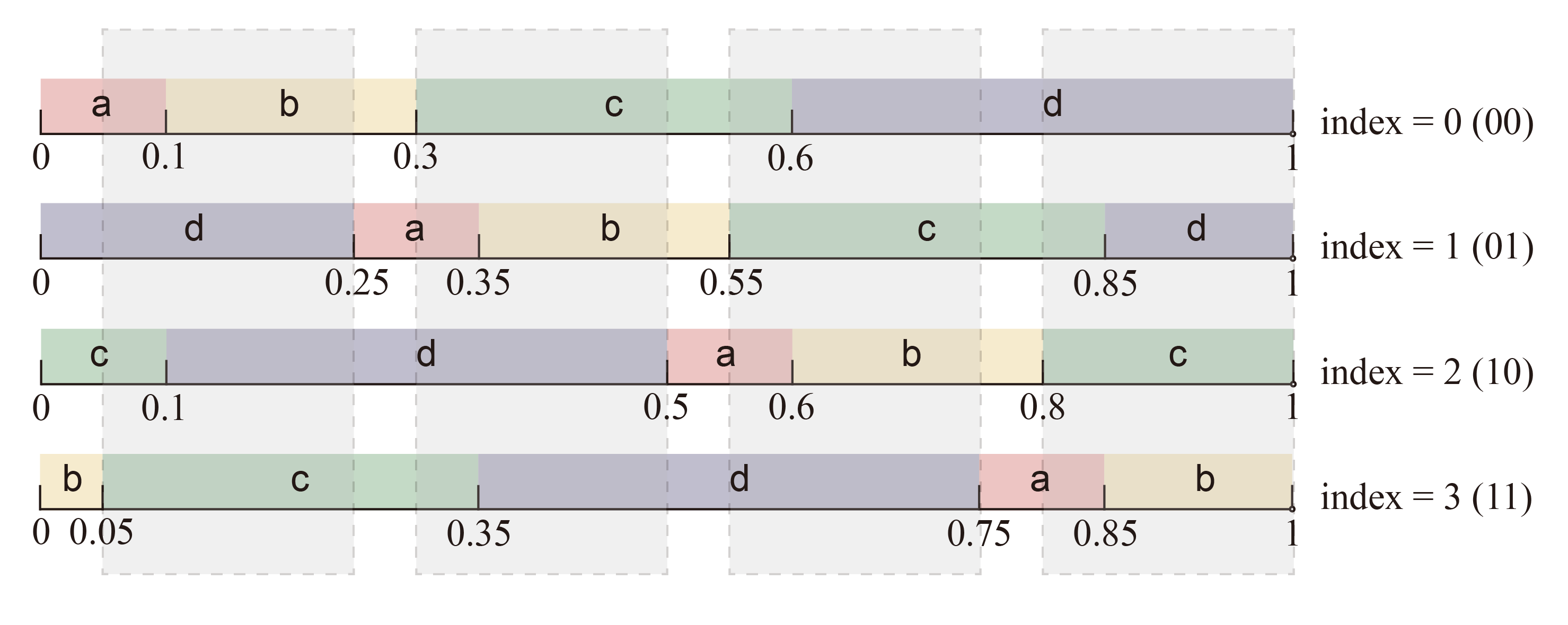
沿用上面的例子,只嵌入 1 比特消息时,无论 PRN 是多少,其在所有分布副本中落入的 token 是互不相同的,因此可以唯一地表达消息;试图嵌入 2 比特消息时,需要创建 $2^{2}=4$ 个分布副本,对应的移位步长为 $1/4=0.25$ ,如下图所示。会出现 PRN 在多个分布副本中落入的 token 相同的情况,我们将这些交集称为争议区间 (disputed ranges) ,如下图中的灰色遮罩覆盖区域所示。当 PRN 不幸落入争议区间中,则无法嵌入 2 比特消息,只能回退到嵌入 1 比特消息的情况。
注意,争议区间的存在并不会影响消息提取的正确性,因为接收方与发送方同步相同的状态,可以计算出争议区间并判断 PRN 是否落入争议区间。因此,他知道发送方嵌入了多少比特消息,可以创建与发送方相同的分布副本来提取消息,并正确地提取消息。
我们推导出,这种构造的嵌入率约等于分布的最小熵 (minimum entropy) 。
嵌入率推导过程可参考 Q1. Detailed description of embedded rate calculation 。
安全性分析
直觉上,载体是从原始分布上进行随机采样得到的,而载密是从原始分布的多个分布副本之一进行随机采样得到的。因为所有分布副本对应的分布是相同的,所以载体分布等于载密分布。
更严格地来说:载密和载体的区别仅在于:采样过程中使用的伪随机数是否经历了循环移位。而根据伪随机数的伪随机性,其在循环移位前后的分布在计算上不可区分。那么,可以推导出载密和载体的分布在计算上不可区分,这就证明了安全性。
更详细的安全性证明可参考 Proof of Security 。
通过递归提升嵌入率
上面提出的基础构造的嵌入率太低,仅仅约等于分布的最小熵,与其理论极限 (分布的熵) 的差距较大,因此,我们进一步研究了如何提高嵌入率。
考虑一个简单的例子,假设有 a、b、c 三种 token ,概率分别为 0.5、0.25、0.25 。如果使用基础构造,那么只能嵌入 1 比特消息。
但如果提前将 b 和 c 放入一个分组 $G$ 中,a 和 $G$ 的概率分别为 0.5 和 0.5 ,使用基础构造一定可以嵌入 1 比特消息。如果选择 $G$ (概率为 0.5 ) ,因为其中的 b 和 c 在归一化后的概率分别为 0.5 和 0.5 ,那么可以再次通过这种构造额外嵌入 1 比特消息。提升后的嵌入容量的期望为 1.5 比特。
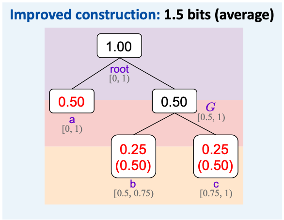
这样,我们可以通过递归分组构建一棵二叉树 (实际选用的是 Huffman 树) ,然后在从根节点走到一个叶子节点的过程 (即若干次子节点选择的过程) 中嵌入消息。实际上,这相当于将原先的一轮多元分布采样分解为多轮二元分布采样,每次采样都可能可以嵌入 1 比特消息。

我们取分布副本的英文 (distribution copies) 中的部分字母,将提升后的构造称为 Discop 。
部署
理论上,Discop 可以部署于任何能给出显式概率分布的生成模型上。为了展示 Discop 对不同媒体生成任务的支持,我们选择了几种典型的生成任务和相应的公开预训练模型来部署 Discop 。
| 任务 | 描述 | 模型 |
|---|---|---|
| 文本生成 | 输入上文,生成其续写。 | GPT-2, DistilGPT-2, Transformer-XL |
| 图像补全 | 输入图像的上半部分,将其补全为完整图像。 | Image GPT |
| 语音合成 | 输入一段文本,合成其对应的语音。 | Tacotron + WaveRNN |
实验评估
实验设置
考虑已在生成任务中广泛使用的 top-$p$ 采样,在截断参数 $p$ 取不同值的情况下开展实验。
在 GPT-2 124M 模型上,将 Discop 与现有的追求可证明安全的隐写方法 ADG、Meteor 进行对比。
Meteor 的初始版本 (下文称为 Meteor w/o sort) 嵌入率较低,因此,其作者设计了一种用于提升嵌入率的启发式排序算法 (下文将提升后的版本直接称为 Meteor) 。我们对 Meteor 的这两种版本都进行了实验。
评估指标
我们主要从安全性和效率 (包括时间效率和容量效率) 进行评估。
- 安全性:$P_{\mathrm{c}}$ 和 $P_{\mathrm{s}}$ 之间的 KL 散度,关注平均值 (Ave KLD) 和最大值 (Max KLD) ,越小越好。
- 时间效率:嵌入一比特消息需要的平均时间,总时间 / 消息总长度,越小越好。
- 容量效率:由于生成过程涉及随机采样,所以嵌入容量的理论极限并不是固定不变的。为了更好地刻画嵌入容量与其理论极限之间的距离,我们提出了一种全新的度量指标——对熵的利用率 (Utilization) ,越大越好。

此外,我们还希望与正常生成相比,隐写的消息嵌入和提取引入的额外时间消耗尽可能少。
实验结果与分析
对比实验
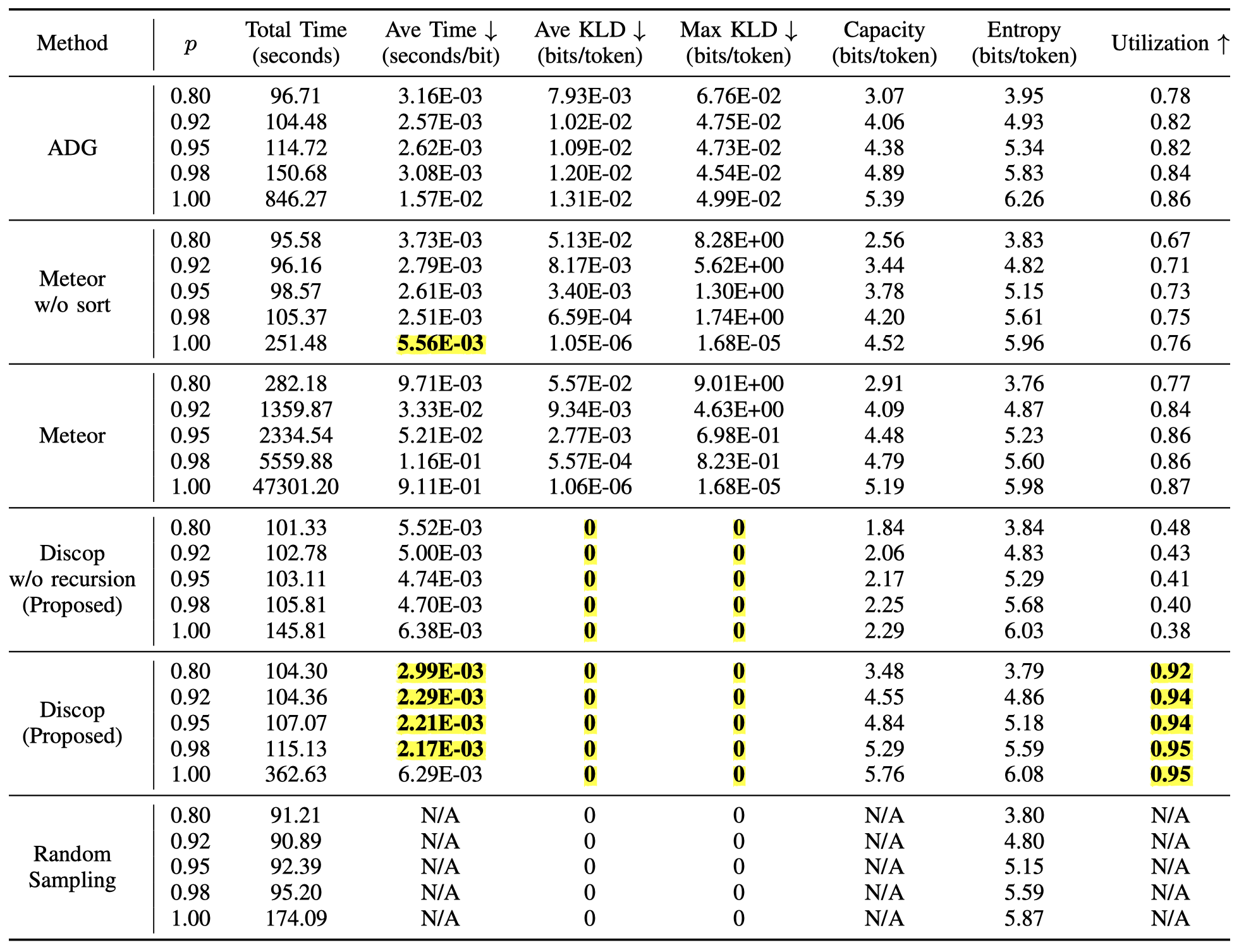
注:Meteor 有两个版本,表中 “Meteor w/o sort” 对应初始版本,“Meteor” 对应引入启发式排序算法提升后的版本。“Discop w/o recursion” 对应我们提出的基础构造。Random Sampling 对应随机采样,即不嵌入消息的正常生成。
总体来看,Discop 在几乎所有指标上都好于之前的方法。
- 安全性:ADG、Meteor 和 Meteor w/o sort 的 KL 散度远远达不到“可忽略”,这可能导致敌手获得区分载体与载密的不可忽略的优势。而 Discop 可以很好地保持分布。
- 时间效率:在 $p$ 取大多数值时,除 Meteor 外的隐写构造都不会引入过多的额外时间。Meteor 引入的启发式排序算法过于复杂,大大增加了其消息嵌入时间——若要嵌入相同长度的消息,Meteor 所需时间是 Discop 的 3.45~144.88 倍,这在需要实时隐写通信的场景可能是无法接受的。
- 容量效率:ADG 和 Meteor 的 Utilization 相当,约为 0.77~0.87 。Meteor w/o sort 的 Utilization 只有约 0.67~0.76 。而 Discop 可以比较充分地利用熵,其 Utilization 达到约 0.92~0.95 。
Discop 引入的额外时间
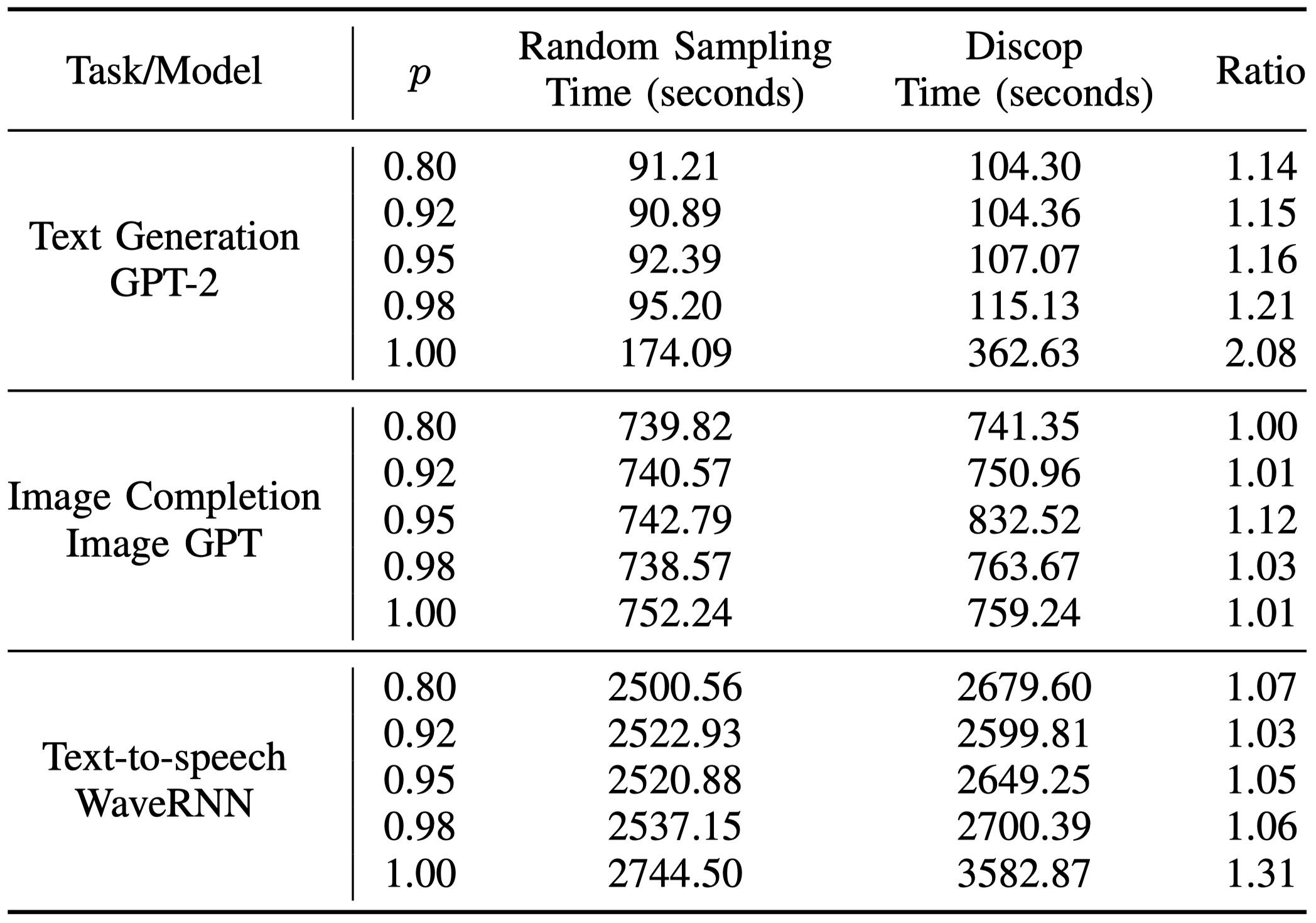
对于候选元素数为 50,257 的 GPT-2 而言,top-$p$ 截断 ($p\ne 1.00$) 去除了大量候选元素,使得额外时间很小。而对于候选元素数为 512 的 Image GPT 和候选元素数为 1024 的 WaveRNN ,不管 $p$ 的取值如何,Discop 引入的额外时间都相对较小。
总结
本文的主要贡献为:
- 分析了之前追求可证明安全的隐写方法在实践中的问题。
- 提出了全新的基于分布副本 (distribution copies) 的可证明安全隐写构造。
- 提出了更合理的容量效率度量指标——对熵的利用率 (Utilization) ,消除了随机性对衡量容量效率的影响。
- 通过递归将嵌入容量提升至其理论极限的约 0.95 ,将提升后的方法命名为 Discop ,这是首个能在实现时保持原始数据分布的高效可证明安全隐写构造。
- 将 Discop 部署于三种典型生成任务上,从安全性和效率两方面开展实验。
我们希望这个工作能为后续的隐私增强技术研究提供基础和灵感。
Jinyang Ding, Kejiang Chen, Yaofei Wang, Na Zhao, Weiming Zhang, and Nenghai Yu. “Discop: Provably Secure Steganography in Practice Based on ‘Distribution Copies’ ”, in 2023 IEEE Symposium on Security and Privacy (SP), IEEE Computer Society, May 2023, pp. 2238–2255. doi: 10.1109/SP46215.2023.10179287.
论文作者:丁锦扬,陈可江,王垚飞,赵娜,张卫明,俞能海
Personal homepage: https://dingjinyang.github.io/
English Version
⚠️ This English version was AI-translated from the Chinese original and is currently under review.
Steganographic Security
In the field of steganography, the pursuit of provable security has a long-standing history.
In 1949, the pioneer of information science, Claud Shannon, clearly pointed out the difficulty of constructing a covert system in his classic paper “Communication Theory of Secrecy Systems”. It wasn’t until the 1990s that the academic community began to define steganographic security by imitating the security definitions in cryptography. In 1998, Christian Cachin gave the definition of information-theoretic security for steganography. He used the KL divergence $D_{\mathrm{KL}}\left(P_{\mathrm{c}}\|P_{\mathrm{s}} \right)$ between the distribution $P_{\mathrm{c}}$ of cover data and the distribution $P_{\mathrm{s}}$ of stego data to model steganographic security. The smaller the KL divergence, the closer $P_{\mathrm{c}}$ and $P_{\mathrm{s}}$ are, and the greater the probability that an adversary makes a wrong judgment, which means the steganographic system is more secure. If $D_{\mathrm{KL}}\left(P_{\mathrm{c}}\|P_{\mathrm{s}} \right)\le\epsilon$, the steganographic system is said to be $\epsilon$-secure. If $\epsilon = 0$, the steganographic system is called perfectly secure. In this case, $P_{\mathrm{c}}$ and $P_{\mathrm{s}}$ are strictly equal, and the adversary’s ability to distinguish whether an object is a cover or stego is no better than random guessing. In 2002, Nicholas Hopper, John Langford, and Luis von Ahn from the team of ACM Turing Award Laureate Prof. Manuel Blum gave the definition of computational security for steganography at CRYPTO 2002. They assumed that the adversary was playing a discrimination game to judge whether an object was a cover or stego. If the attack advantages of all probabilistic polynomial-time (PPT) adversaries are negligible with respect to the security parameter, the steganographic system is considered secure.
Definitions:
- Cover: an object without a secret message embedded
- Stego: an object with a secret message embedded
References:
- C. E. Shannon. Communication Theory of Secrecy Systems. BSTJ ’49
- C. Cachin. An Information-Theoretic Model for Steganography. IH ’98
- N. J. Hopper et al. Provably Secure Steganography. CRYPTO ’02
Side note: Christian Cachin is an IACR Fellow and one of the initiators of the Cryptology ePrint Archive (which can be understood as the arXiv in the field of cryptography). Luis von Ahn is the first author of CAPTCHA and one of the founders of Duolingo.
Why Do We Need Provably Secure Steganography
Translation of the dialogue in the picture:
- Bob: Steganography is a very secure method of communication.
- Alice: Is it provably secure?
- Bob: It is secure in real-world applications.
- Alice: I know, but is it provably secure?
- Bob: Can you crack it?
- Alice: No, but is it provably secure?
- Bob: …
You can refer to Section 1: Empirical Security and Provable Security of Steganography in the Chinese paper “Provably Secure Steganography: Theory, Applications, and Prospects” .
……
For an empirically secure steganographic algorithm, the attacker always has a considerable advantage, even if it is relatively small. Therefore, for steganographers, there is a significant risk when using this steganographic tool because the attacker can identify them with very high confidence through a certain amount of data. Steganographers will then think about how to make the attacker’s advantage zero or negligible. This actually corresponds to provably secure steganography. If we can ensure that the advantage obtained by an attacker with any computational ability is zero without limiting the attacker’s computational ability, this is called information-theoretic security. If we take a step back and can ensure that the advantage obtained by an attacker with limited computational ability is negligible, this is computationally secure steganography.
Existing Provably Secure Steganographic Constructions and Their Problems in Practice
Since the definition of steganographic security was proposed, researchers have successively proposed several steganographic constructions aiming for provable security. We analyzed their problems in practice.
- Construction based on rejection sampling: The expected time consumption increases exponentially with the length of the embedded message. When the min-entropy of the distribution is very small, the rejection sampling algorithm is extremely likely to fail.
- Construction based on arithmetic coding: The probability of any message has the form of $2^{-l}\left(l\in \mathbb{N} \right)$, and correspondingly, the stego data also has the form of $2^{-l}$. However, it is almost impossible for the cover data distribution predicted by the model to exactly match this stego data distribution. This requires the message embedding algorithm to modulate the cover data distribution, thus introducing distortion. To reduce the distortion, we can simply increase the message length by padding, making the probability of the cover data smaller and closer to a certain $2^{-l}$. As the message length approaches infinity, the distortion tends to 0, which is obviously impractical. Even so, the introduced distortion is a negligible function of the message length (rather than the security parameter), making this construction unable to achieve the expected security.
- Construction based on grouping: This construction is secure if and only if the grouping is perfectly balanced. However, it is difficult to balance the grouping of discrete probability distributions, making this construction unable to achieve the expected security.
References:
- N. J. Hopper et al. Provably Secure Steganography. CRYPTO ’02
- L. von Ahn and N. J. Hopper. Public-Key Steganography. EUROCRYPT ’04
- M. Backes and C. Cachin. Public-Key Steganography with Active Attacks. TCC ’05
- T. V. Le. Efficient Provably Secure Public Key Steganography. Cryptology ePrint Archive ’03
- K. Yang et al. Provably Secure Generative Steganography Based on Autoregressive Model. IWDW ’18
- Z. Ziegler et al. Neural Linguistic Steganography. EMNLP ’19
- K. Chen et al. Distribution-Preserving Steganography Based on Text-to-Speech Generative Models. TDSC ’21
- G. Kaptchuk et al. Meteor: Cryptographically Secure Steganography for Realistic Distributions. CCS ’21
- S. Zhang et al. Provably Secure Generative Linguistic Steganography. ACL Findings ’21
Provably Secure Steganographic Construction Based on Distribution Copies
In this paper, we propose a new provably secure steganographic construction based on distribution copies.
We take the text generation task as an example to introduce the proposed steganographic construction. This type of task generally uses an auto-regressive model such as the GPT series models to generate text token by token. Specifically, given a context as input, the auto-regressive model will predict the probability distribution $\mathcal{P}^{(t)}=\Pr \left[x_{t}\mid x_{<t} \right]$ of the next token, and then randomly sample a token from this probability distribution as the next token to be appended to the end of the context. Repeat the prediction and random sampling until the termination condition is met.
Random sampling is generally implemented through the following steps:
- On the interval $\left[0,1 \right)$, allocate non-overlapping left-closed and right-open intervals to all candidate tokens according to $\mathcal{P}^{\left(t \right)}$. The length of the interval corresponding to each token is equal to the probability that this token is selected.
- Consume a pseudo-random number (PRN) $r^{\left(t \right)}$ generated by a pseudo-random number generator (PRNG), and select the token corresponding to the interval in which $r^{\left(t \right)}$ falls as the next token.
Example: Suppose $r^{\left(t \right)} = 0.937$. Since it falls into the interval corresponding to “dear”, we select “dear” as the next token.
How to securely embed a message during the generation process?
We believe that the answer to this question is to perform sampling under the control of the secret message. This sampling needs to meet two conditions:
- Indistinguishable: The steganographic sampling should be indistinguishable from random sampling.
- Reversible: The receiver can decode the received tokens into the secret message.
Basic Construction
We observe that for a probability distribution with more than one candidate token, the interval allocation scheme is not unique.
Thus, given a probability distribution, we can create multiple distribution copies for it and then use the index value of the distribution copies to represent the message.
We create distribution copies through rotation. To facilitate understanding, here is an example.
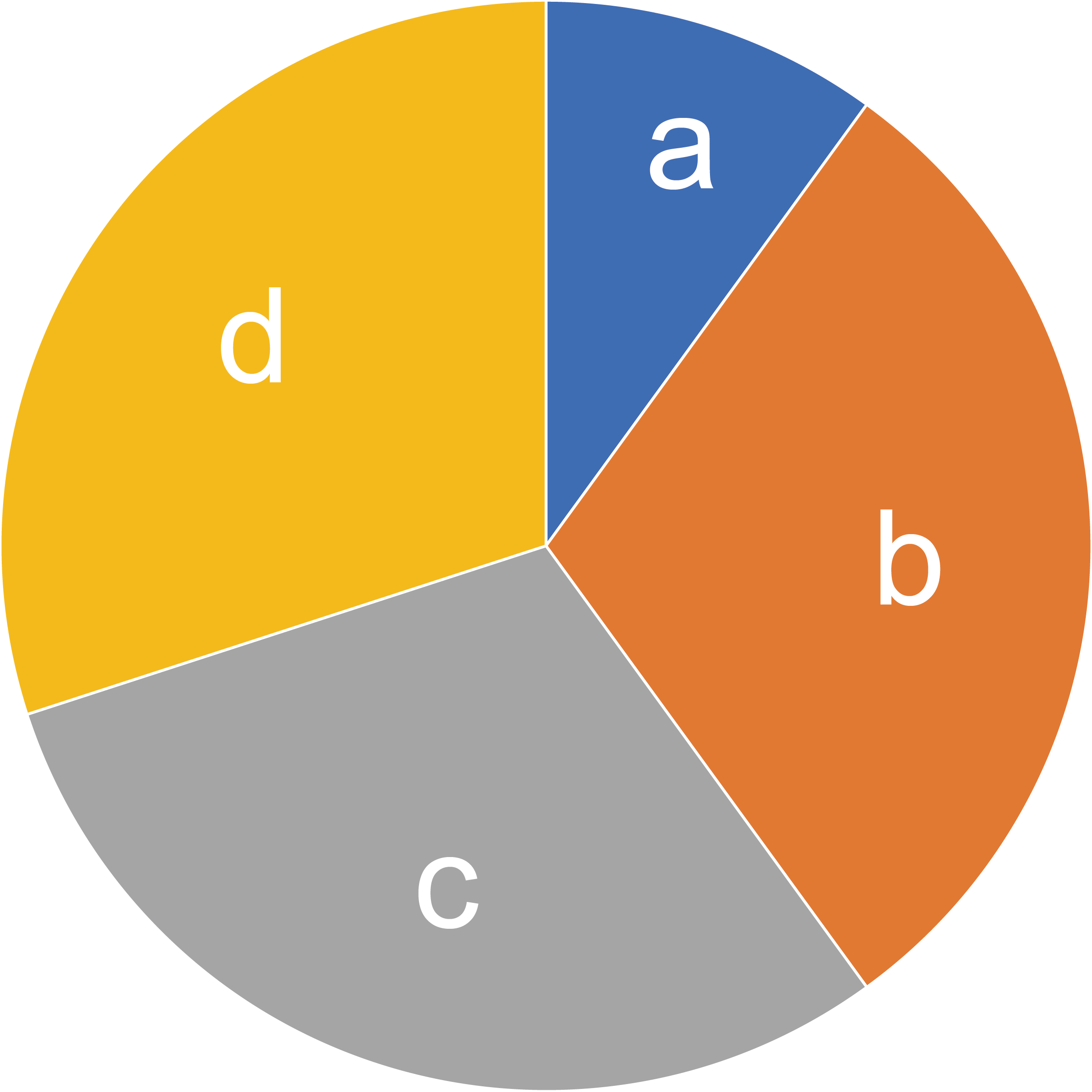
Suppose the probability distribution is as follows:
Let the allocation scheme arranged in the order of “a-b-c-d” be the initial interval allocation scheme, that is, distribution copy 0.
If we want to embed 1 bit of message, we need to create $2^{1}=2$ distribution copies, and the corresponding shift step is $1/2 = 0.5$.
By rotating distribution copy 0 by 0.5, we can get distribution copy 1.
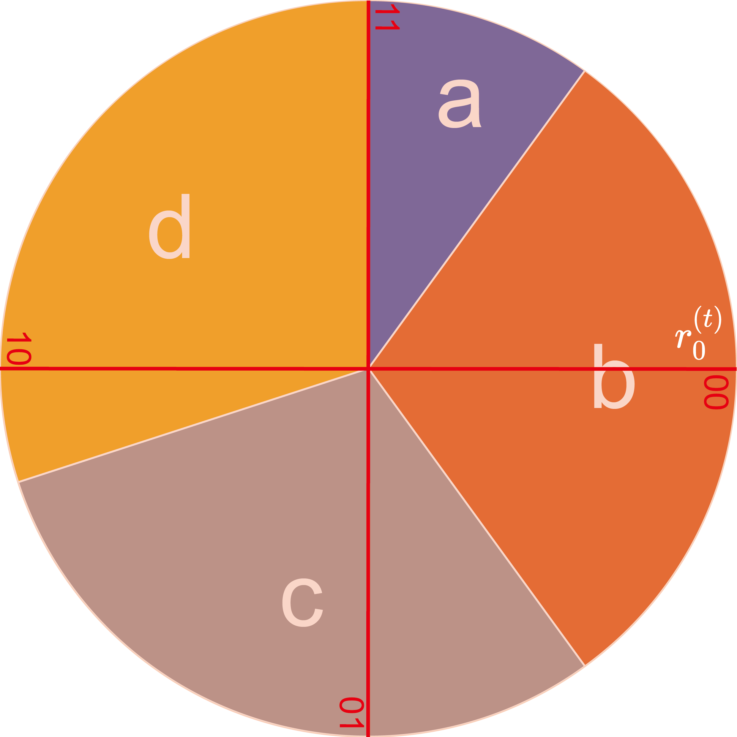
Suppose the PRN $r^{\left(t \right)}$ generated by the PRNG is 0.2.
- If the message $m = 0$, we sample from distribution copy 0. Since $r^{\left(t \right)}$ falls into the interval corresponding to “b”, we sample “b” as the next token.
- If the message $m = 1$, we sample from distribution copy 1. Since $r^{\left(t \right)}$ falls into the interval corresponding to “d”, we sample “d” as the next token.
🤔️ How does the receiver extract the message?
If the receiver shares the same context and generative model with the sender, he can obtain the same probability distribution. Similarly, if the receiver shares the same seed and PRNG with the sender, he can obtain the same PRN.
In this way, the receiver can synchronize the same state as the sender and extract the message by judging from which distribution copy the received token was sampled.
Unique Decoding Condition, Disputed Ranges, and Embedding Rate
How to ensure that the receiver can correctly extract the message? How long a message can be embedded?
It is not difficult to deduce that only when the tokens corresponding to the intervals in which the consumed PRN falls in all distribution copies (hereinafter referred to as “the fallen tokens”) are different from each other can this sampling uniquely represent the message.
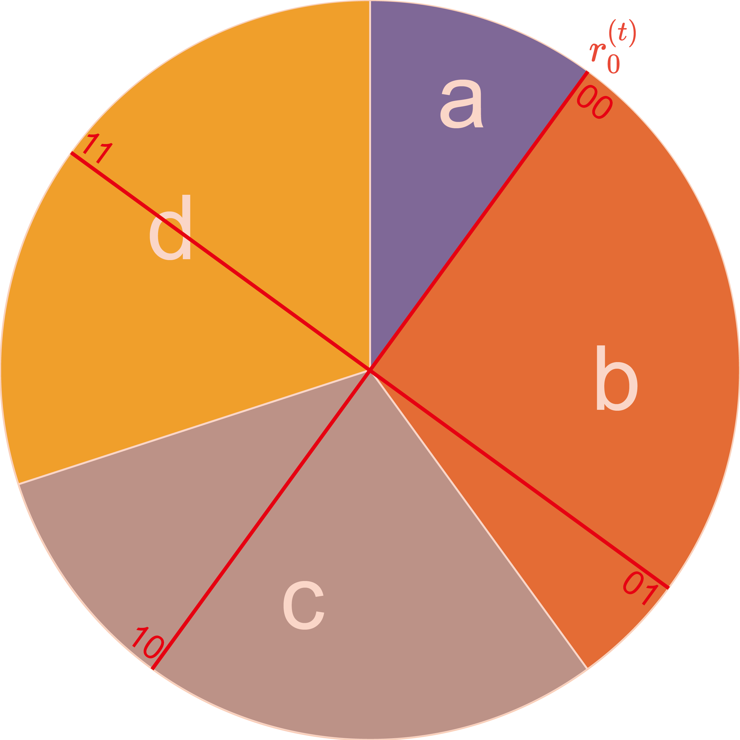
Using the above example, when only 1 bit of message is embedded, no matter what the PRN is, the fallen tokens in all distribution copies are different from each other, so the message can be uniquely represented. When trying to embed 2 bits of message, we need to create $2^{2}=4$ distribution copies, and the corresponding shift step is $1/4 = 0.25$, as shown in the following figure. There will be cases where the PRN falls into the same token in multiple distribution copies. We call these intersections disputed ranges, as shown by the gray-shaded areas in the following figure. When the PRN unfortunately falls into the disputed range, we cannot embed 2 bits of message and can only fall back to the case of embedding 1 bit of message.
Note that the existence of the disputed range does not affect the correctness of message extraction because the receiver and the sender synchronize the same state, can calculate the disputed range, and judge whether the PRN falls into the disputed range. Therefore, he knows how many bits of message the sender has embedded, can create the same distribution copies as the sender to extract the message, and correctly extract the message.
We derived that the embedding rate of this construction is approximately equal to the minimum entropy of the distribution.
The derivation process of the embedding rate can be found in Q1. Detailed description of embedded rate calculation.
Security Analysis
Intuitively, a cover is obtained by random sampling from the original distribution, while a stego is obtained by random sampling from one of the multiple distribution copies of the original distribution. Since the distributions corresponding to all distribution copies are the same, the cover distribution is equal to the stego distribution.
More strictly speaking, the only difference between a stego and a cover is whether the pseudo-random number used in the sampling process has undergone rotation. According to the pseudo-randomness of the pseudo-random number, the distributions before and after rotation are computationally indistinguishable. Then, we can deduce that the distributions of the stego and the cover are computationally indistinguishable, which proves the security.
A more detailed security proof can be found in Proof of Security.
Improving the Embedding Rate through Recursion
The embedding rate of the basic construction proposed above is too low, only approximately equal to the minimum entropy of the distribution, and there is a large gap between it and the theoretical limit (the entropy of the distribution). Therefore, we further studied how to improve the embedding rate.
Consider a simple example. Suppose there are three types of tokens: “a”, “b”, and “c”, with probabilities of 0.5, 0.25, and 0.25 respectively. If we use the basic construction, we can only embed 1 bit of message.
However, if we put “b” and “c” into a group $G$ in advance, and the probabilities of “a” and $G$ are 0.5 and 0.5 respectively, we can definitely embed 1 bit of message using the basic construction. If we choose $G$ (with a probability of 0.5), since the normalized probabilities of “b” and “c” in it are 0.5 and 0.5 respectively, we can embed an additional 1 bit of message through this construction again. The expected improved embedding capacity is 1.5 bits.
In this way, we can construct a binary tree (actually a Huffman tree) through recursive grouping and then embed the message during the process of walking from the root node to a leaf node (that is, the process of several child-node selections). In fact, this is equivalent to decomposing the original one-round multi-distribution sampling into multiple rounds of binary-distribution sampling, and each sampling may be able to embed 1 bit of message.
We take some letters from the English of distribution copies and name the improved construction Discop.
Deployment
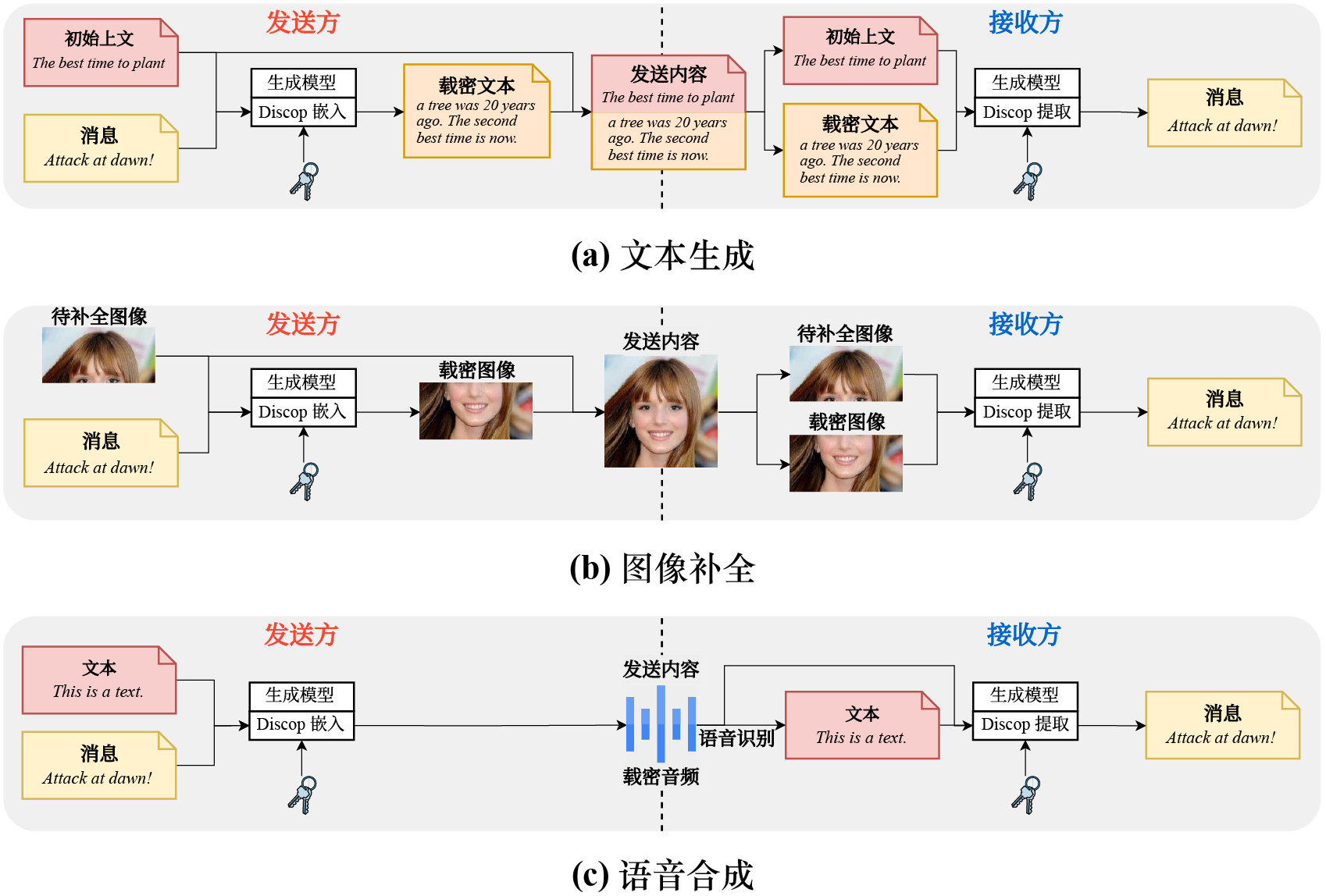
Theoretically, Discop can be deployed on any generative model that can give an explicit probability distribution. To demonstrate Discop’s support for different media generation tasks, we selected several typical generation tasks and corresponding publicly available pre-trained models to deploy Discop.
| Task | Description | Models |
|---|---|---|
| Text Generation | Given a context, write a continuation of it. | GPT-2, DistilGPT-2, Transformer-XL |
| Image Completion | Given part of an image (e.g., the upper half part), complete it. | Image GPT |
| Text-to-Speech | Given a piece of text, synthesize its corresponding speech. | Tacotron + WaveRNN |

Experimental Evaluation
Experimental Setup
Considering the top-$p$ sampling widely used in generation tasks, we conducted experiments with different values of the truncation parameter $p$.
On the GPT-2 124M model, we compared Discop with the existing steganographic methods ADG and Meteor that aim for provable security.
The initial version of Meteor (hereinafter referred to as Meteor w/o sort) has a lower embedding rate. Therefore, its authors designed a heuristic sorting algorithm to improve the embedding rate (the improved version is directly referred to as Meteor hereinafter). We conducted experiments on both versions of Meteor.
Evaluation Metrics
We mainly evaluated from the aspects of security and efficiency (including time efficiency and capacity efficiency).
- Security: The KL divergence between $P_{\mathrm{c}}$ and $P_{\mathrm{s}}$, focusing on the average value (Ave KLD) and the maximum value (Max KLD). The smaller, the better.
- Time Efficiency: The average time required to embed 1 bit of message, which is the total time divided by the total message length. The smaller, the better.
- Capacity Efficiency: Since the generation process involves random sampling, the theoretical limit of the embedding capacity is not fixed. To better characterize the distance between the embedding capacity and its theoretical limit, we proposed a brand-new metric-the utilization rate of entropy (Utilization). The larger, the better.
In addition, we also hope that the additional time consumption introduced by message embedding and extraction in steganography is as small as possible compared with normal generation.
Experimental Results and Analysis
Comparative Experiment
Note: Meteor has two versions. In the table, “Meteor w/o sort” corresponds to the initial version, and “Meteor” corresponds to the version improved by introducing the heuristic sorting algorithm. “Discop w/o recursion” corresponds to the basic construction we proposed. Random Sampling corresponds to random sampling, that is, normal generation without message embedding.
Overall, Discop performs better than previous methods in almost all metrics.
- Security: The KL divergences of ADG, Meteor, and Meteor w/o sort are far from being “negligible”, which may give the adversary a non-negligible advantage in distinguishing between covers and stegos. In contrast, Discop can well maintain the distribution.
- Time Efficiency: When $p$ takes most values, except for Meteor, the steganographic constructions do not introduce excessive additional time. The heuristic sorting algorithm introduced by Meteor is too complex, greatly increasing its message embedding time. To embed the same length of message, Meteor takes 3.45 - 144.88 times as long as Discop, which may be unacceptable in scenarios requiring real-time steganographic communication.
- Capacity Efficiency: The Utilization values of ADG and Meteor are quite similar, approximately 0.77 - 0.87. The Utilization of Meteor w/o sort is only about 0.67 - 0.76. In contrast, Discop can make relatively full use of entropy, and its Utilization reaches about 0.92 - 0.95.
Additional Time Introduced by Discop
For GPT-2 with 50,257 candidate elements, top-$p$ truncation ($p\ne 1.00$) removes a large number of candidate elements, making the additional time very small. For Image GPT with 512 candidate elements and WaveRNN with 1024 candidate elements, regardless of the value of $p$, the additional time introduced by Discop is relatively small.
Conclusion
The main contributions of this paper are as follows:
- Analyzed the problems of previous steganographic methods aiming for provable security in practice.
- Proposed a new provably secure steganographic construction based on distribution copies.
- Proposed a more reasonable metric for capacity efficiency termed “Utilization”, mitigating the interference of randomness in the assessment of capacity-efficiency.
- Improved the embedding capacity to about 0.95 of its theoretical limit through recursion and named the improved method Discop, which is the first efficient and provably secure steganography algorithm that preserves the original data distribution in practice.
- Deployed Discop on three typical generation tasks and conducted experiments from the aspects of security and efficiency.
We hope that this work can provide a foundation and inspiration for subsequent research on privacy-enhancing technologies.
Jinyang Ding, Kejiang Chen, Yaofei Wang, Na Zhao, Weiming Zhang, and Nenghai Yu. “Discop: Provably Secure Steganography in Practice Based on ‘Distribution Copies’ ”, in 2023 IEEE Symposium on Security and Privacy (SP), IEEE Computer Society, May 2023, pp. 2238–2255. doi: 10.1109/SP46215.2023.10179287.
Authors: Jinyang Ding, Kejiang Chen, Yaofei Wang, Na Zhao, Weiming Zhang, and Nenghai Yu
Personal homepage: https://dingjinyang.github.io/
Errata
Fig. 2
In Fig. 2, the method rotate all intervals to the right by $d$, which is equivalent to rotating the consumed pseudo-random number to the left by $d$. However, in rest of this paper, the rotation direction is opposite: rotating all intervals to the left by $d$, which is equivalent to rotating the consumed pseudo-random number to the right by $d$.
Considering that the rotation direction is irrelevant to the correctness of the method description, there is nothing factually wrong with Fig. 2 itself. However, to prevent any potential confusion for readers due to the inconsistency, it would be advisable to modify Fig. 2 to align it with the rest.
Before modification:
After modification:
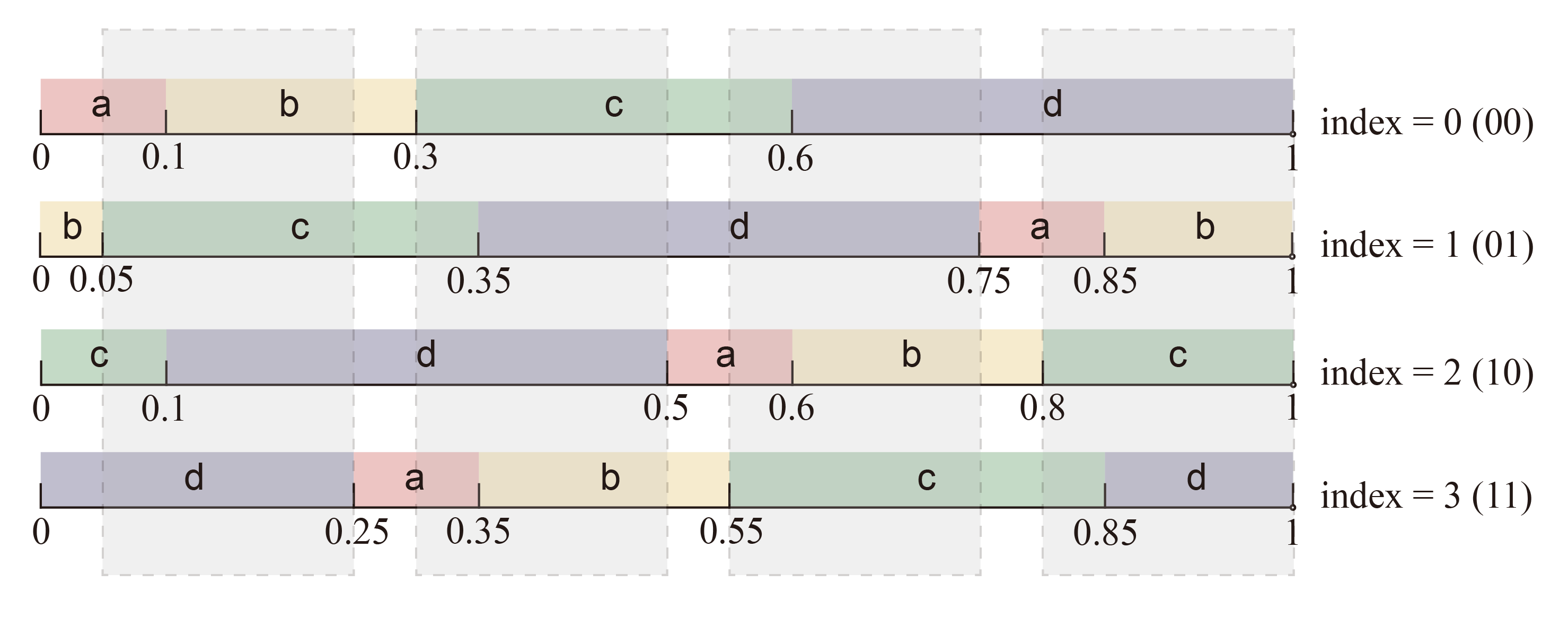
Accordingly, Paragraph 1 on Page 6 (the paragraph on the left of Fig. 2) requires an amendment: in the “distribution copies” with index 0 and 1 → in the “distribution copies” with index 0 and 3.
Proof of Security
Thanks to Xin Zhang and Zirui Wang for providing valuable advice on the new version of proof of security! 🤗
The security proof in the paper was a bit inaccurate, so we reconsider the security proof. In the following, we will first review the definition of PRNG and introduce how to use a PRNG to generate real numbers in $[0,1)$, and then give the security proof of the steganography method based on “distribution copies”.
Definition of PRNG
Reference: Katz and Lindell. Introduction to Modern Cryptography, Second Edition. Chapman and Hall/CRC. 2014.
Let $G$ be a deterministic polynomial-time algorithm such that for any $\lambda$-bit input $s \in \{0, 1\}^\lambda$, the algorithm $G$ outputs a bit string of length $\ell(\lambda)$, where $\ell$ is a polynomial. If $G$ satisfies the following two conditions, it is referred to as a (computationally secure) pseudo-random number generator (PRNG):
- Expansion: For all $\lambda$, it holds that $\ell(\lambda) > \lambda$.
- Pseudo-randomness: For all probabilistic polynomial-time distinguishers $\mathcal{A}$, there exists a negligible function $\operatorname{negl}$ such that the following inequality holds:Where the seed $s$ is uniformly chosen from $\{0, 1\}^\lambda$, and $s’$ is uniformly chosen from $\{0, 1\}^{\ell(\lambda)}$, both being true random bit strings.
How can a PRNG be used to generate a real number in the interval $[0,1)$? Assume the PRNG outputs a bit string $G(s) = b_0, b_1, \ldots, b_i, \ldots, b_{\ell(\lambda)-1}$, where $b_i \in \{0, 1\}$. At each time step $t$, consecutive $h$ bits $b_{ht}, b_{ht+1}, \ldots, b_{ht+h-1}$ are sequentially taken from $G(s)$, and by calculating
a pseudo-random number $r^{(t)} \in [0,1)$ within the interval $[0,1)$ can be obtained, where $h$ can be referred to as the precision of the pseudo-random number.
Proof of Security
To demonstrate that the stego distribution is computationally indistinguishable from the cover distribution, it suffices to prove that the random variables used in these two sampling processes are computationally indistinguishable, given that the only difference between the stego and the cover lies in the random variables used during the sampling process.
At any time step $t$, suppose a message $m^{(t)}$ of length $n_{t}$ bits is to be embedded. According to the fundamental axioms of probability theory, the sum of the probabilities of all possible values of the message $m^{(t)}$ equals 1, that is,
The sender employs a computationally secure PRNG to generate a pseudo-random bit string $b_{ht}, b_{ht+1}, \ldots, b_{ht+h-1}$, which is then transformed into a real number $r^{(t)}\in\left[0,1\right)$ with precision $h$ (where $h \geq n_{t}$). Thus, for all $a \in \left\{i \times 2^{-h}\right\}_{i=0,\dots,2^h-1}$, there exists a negligible function $\varepsilon$ with respect to the security parameter $\lambda$ such that the following inequality holds:
Therefore,
In practice, $r^{(t)}$ can be considered as the random variable used for normal sampling. Let $r^{\prime(t)}$ be the random variable used for steganographic sampling, $\textsf{dcm}(m)$ be the decimal representation of the message $m$, and $z(a, m) = \textsf{rotate}(a, -\textsf{dcm}(m) \times 2^{-n_t}, 1)$ denote the value obtained by rotating $a$ to the left within the interval $[0,1)$ by $\textsf{dcm}(m) \times 2^{-n_t}$. Then, for $a \in \{i \times 2^{-h}\}_{i=0,\dots,2^h-1}$ and $m \in \{0, 1\}^{n_t}$, we have
Since $h$ is a constant independent of $\lambda$, there exists a negligible function $\varepsilon^{\prime}\left(\lambda\right) = 2^{h+1} \cdot \varepsilon\left(\lambda\right)$ with respect to $\lambda$ such that the following inequality holds:
Given that the only difference between the stego and the cover is the random variable used during the sampling process, and the distributions of $r^{\prime(t)}$ (the random variable used for steganographic sampling) and $r^{(t)}$ (the random variable used for normal sampling) are computationally indistinguishable, it follows that the stego and cover distributions are also computationally indistinguishable.
Therefore, all of Discop’s KLDs in Table II should be changed to “negligible”? 🤔
Minor
Page 2, inconsistent format: c) Efficient Attempts to Provably Secure Steganography → c) Efficient attempts to provably secure steganography.
Page 10, Algorithm 3:
- $r_0\le\mathrm{separator}$ → $r_0<\mathrm{separator}$
- $r_1\le\mathrm{separator}$ → $r_1<\mathrm{separator}$
Q&A
Q1. Detailed description of embedded rate calculation
On the bottom left corner of Page 6, you mentioned:
We denote the maximum token probability at time step $t$ as $p_{\max}^{(t)}$ , and the theoretical upper bound of $\beta^{(t)}$ as $\mathrm{B}^{(t)}$. According to the condition for unique decoding, it can be deduced that $p_{\max}^{(t)}/2<2^{-\mathrm{B}^{(t)}}\le p_{\max}^{(t)}$ , and $\beta^{(t)}=\left\lfloor \mathrm{B}^{(t)} \right\rfloor\in \mathbb{N}$, so
Can you give a more detailed description?
A1
To understand $p_{\max}^{(t)}/2<2^{-\mathrm{B}^{(t)}}\le p_{\max}^{(t)}$, you need some imagination. The instantaneous embedding rate must be in integer bits, so $\beta^{(t)}\in\mathbb{N}$. To facilitate derivation, here we denote its theoretical upper bound as $\mathrm{B}^{(t)}\in\mathbb{R}$.
Overall, the two parts of the inequality $p_{\max}^{(t)}/2<2^{-\mathrm{B}^{(t)}}\le p_{\max}^{(t)}$ correspond to two extreme cases respectively.
Perhaps it would be easier to comprehend this using a pie chart, where the central angle of each slice is directly proportional to a token probability. Suppose there are four tokens, namely “a”, “b”, “c”, and “d”, with probabilities of 0.1, 0.3, 0.3, and 0.3, respectively.
We use line segments (in red) with one end at the origin of the circle and the other end on the circumference of the circle to represent the consumed pseudo-random number and its rotated values.
Now please recall to the condition for unique decoding:
When the tokens sampled by the consumed pseudo-random number from all “distribution copies” are different from each other, the receiver can uniquely decode the message.
To satisfy the condition, there should not be two or more line segments on each slice of the pie chart. In fact, we only need to focus on the maximum probability $p_{\max}^{(t)}$, because if there is only one line segment on the slice corresponding to the most probable token, then there must not be two or more line segments on any other single slice. In the following, we denote the slice corresponding to the most probable token as $s$.
The key point is that if there is already a line segment placed on $s$, its adjacent line segments cannot also be on $s$. When $\mathrm{B}^{(t)}$ reaches its maximum, the corresponding theoretical rotation step $2^{-\mathrm{B}^{(t)}}$ is at its minimum. $2^{-\mathrm{B}^{(t)}}>p_{\max}^{(t)}/2$ corresponds to an extreme case where a line segment is precisely placed at the center of $s$. In this case, the line segment is equidistant from both the start and end points of the slice, with the distances of $p_{\max}^{(t)}/2$ each. To ensure that its adjacent line segments fall outside of $s$, it must hold true that $2^{-\mathrm{B}^{(t)}}>p_{\max}^{(t)}/2$. Please note that due to the intervals being left-closed and right-open, the equal sign cannot be achieved.
$2^{-\mathrm{B}^{(t)}}\le p_{\max}^{(t)}$ corresponds to the other extreme case where a line segment is precisely placed at the start point of $s$. In this case, $2^{-\mathrm{B}^{(t)}}$ reaches its maximum when the next line segment is precisely placed at the start point of the subsequent slice, so $2^{-\mathrm{B}^{(t)}}\le p_{\max}^{(t)}$.
It crucial to emphasize that $\mathrm{B}^{(t)}$ signify the maximum value of the amount of information that can be embedded at time step $t$, since it is meaningless to discuss a scenario where the method allows embedding $m$ bits but only $n$ bits are embedded ($m>n$). If you speak Chinese, you can understand it as “应嵌尽嵌” (meaning “embed as much as possible”). Without a line segment on $s$, there would be an underutilization of the embedding rate.
Given $\beta^{(t)}=\left\lfloor \mathrm{B}^{(t)} \right\rfloor\in \mathbb{N}$, it readily follows that
See Also
Provably Secure Steganography | ComyDream Studio
本文采用 CC BY-NC-SA 4.0 许可协议,转载请注明来自 ComyDream 。
本文链接:http://comydream.github.io/2023/06/07/discop-sp23/